
This is about how the bytes of a data type are arranged in memory. An int variable for example occupies 4 bytes in memory. In case of little endian, the least significant byte of the integer value will be first in memory (at a smaller address). In case of big endian, the most significant byte if the integer value will be the first byte in memory.
Consider the following code that prints the digits of a number by remembering the last digit and by shifting to the left. ‘size’ is the number of bits to print, ‘val’ is the number to print:
void PrintBinary(int val, int size) { unsigned char* b = new unsigned char[size]; memset(b, 0, size); int pos = size – 1; while ( val != 0 ) { b[pos] = val % 2; val = val >> 1; pos–; if (pos < 0) break; } for (pos = 0; pos< size; ++pos) { printf(“%d”, b[pos]); if (pos%8 == 7) printf(” “); } delete[] b; } int x = 8;PrintBinary(x, 32);
Then the above code will print: 00000000 00000000 00000000 00001000
The code below will print ‘00001000 00000000 00000000 00000000’ which shows that it was run on a little endian machine because the least significant byte is first.
unsigned char* b = (unsigned char*) &x;for (int i = 0; i
{ PrintBinary(b[i], 8); }
Here is a method to determine the endianess of a machine:
bool IsLittleEndian(){ int b = 1;
return ((unsigned char*)(&b))[0]; }
A more interesting approach is to use a union (a C++ facility to agregate mode data types over the same memory space):
bool IsLittleEndian(){ union local_t
{ int i;
unsigned char b; };
local_t u;
u.i = 1;
return u.b; }
That was the C++ approach. Java offers an API for it:
import java.nio.ByteOrder;…
if (ByteOrder.nativeOrder().equals(ByteOrder.BIG_ENDIAN)) {
System.out.println(“Big-endian”);
} else {
System.out.println(“Little-endian”);
}
…
In C# the BitConverter class has the IsLittleEndian static method.
 multiples of
  and
and  multiples of
  . Some of those numbers are multiple of both
  ). When summing, we need to avoid summing twice we need to subtract those numbers.
 multiples of
 real matrix
  can be decomposed as:
  where
where  is a
is a  orthogonal matrix,
  is a
is a  is a
is a  orthogonal matrix.
 happens to be a
  , and
, and  .
.  because:
 is grater or equal to
  for some vector
  , it follows that
  when
when  (i.e.
(i.e.  is in the null space of
  otherwise.
 , multiplying
  and considering that
  are orthogonal unit vectors, we get:
 =>
=> =>
=>
 we get:
  =>
=>![A[v_1 ... v_r v'_{r+1} ... v'_{n}]=[u_1 ... u_r u'_{r+1} ... u'_{m}]\begin{bmatrix} {\sqrt \lambda_1} & \cdots & 0 & \cdots & 0 \\ \vdots & \ddots & \vdots & & \vdots \\ 0 & \cdots & {\sqrt \lambda_r} & \cdots & 0 \\ \vdots & & \vdots & & \vdots & \\ 0 & \cdots & 0 & \cdots & 0 \end{bmatrix}](https://s0.wp.com/latex.php?latex=A%5Bv_1+...+v_r+v%27_%7Br%2B1%7D+...+v%27_%7Bn%7D%5D%3D%5Bu_1+...+u_r+u%27_%7Br%2B1%7D+...+u%27_%7Bm%7D%5D%5Cbegin%7Bbmatrix%7D+%7B%5Csqrt+%5Clambda_1%7D+%26+%5Ccdots+%26+0+%26+%5Ccdots+%26+0+%5C%5C+%5Cvdots+%26+%5Cddots+%26+%5Cvdots+%26++%26+%5Cvdots+%5C%5C+0+%26+%5Ccdots+%26+%7B%5Csqrt+%5Clambda_r%7D+%26+%5Ccdots+%26+0+%5C%5C+%5Cvdots+%26++%26+%5Cvdots+%26++%26+%5Cvdots+%26++%5C%5C+0+%26+%5Ccdots+%26+0+%26+%5Ccdots+%26+0+%5Cend%7Bbmatrix%7D&bg=ffffff&fg=333333&s=0&c=20201002)
 is the rank of the matrix.
 to form a basis in
  .
. is extended by the set of orthogonal vectors
  to form a basis in
  .
. symmetric,
  orthogonal (
 ) and
) and  diagonal, such that
 its complement (
 ). If
). If  ,
,  then: for

 .
. and
and  because
  because
  ,
,  and
and  , such that
  .
. is the vector space generated by
  (this can be proven by changing the basis). This means that exists
  such that
  . Considering the vector space generated by
  , and by applying the operator
  . By induction we get:
 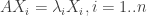 , where the vectors
  are pair wise perpendicular:
  .
.![A[X_1 X_2 ... X_n]=[X_1 X_2 ... X_n]diag(\lambda_1, \lambda_2, ... ,\lambda_n)](https://s0.wp.com/latex.php?latex=A%5BX_1+X_2+...+X_n%5D%3D%5BX_1+X_2+...+X_n%5Ddiag%28%5Clambda_1%2C+%5Clambda_2%2C+...+%2C%5Clambda_n%29&bg=ffffff&fg=333333&s=0&c=20201002)
 , where the columns of
  are the vectors
  . P is orthogonal because vectors
  .
. . I will show in this post that a real symmetric matrix have real eigenvalues.
 and
and  :
: 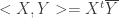 , where
  is the complex conjugate of the vector
  , for any matrix
 .
. and considering that A is symmetric
  .
. and because
  is zero, so the eigenvalue is a real number.